Code examples
Dry mass computation with radial inclusion factor
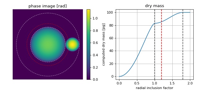
This examples illustrates the usage of the “radial inclusion factor”
which is defined in the configuration section “sphere” and used in
drymass.anasphere.relative_dry_mass() with the
keyword argument rad_fact.
The phase image is computed from two spheres whose dry masses add up to 100pg with the larger sphere having a dry mass of 83pg. The larger sphere is located at the center of the image which is also used as the origin for dry mass computation. The radius of the larger sphere is known (10µm). Thus, the corresponding radius (inner circle) corresponds to a radial inclusion factor of 1. In DryMass, the default radial inclusion factor is set to 1.2 (red). In some cases, this inclusion factor must be increased or decreased depending on whether additional information (the smaller sphere) should be included in the dry mass computation or not.
mass_radial_inclusion_factor.py
 1from drymass.anasphere import relative_dry_mass
 2import matplotlib
 3import matplotlib.pylab as plt
 4import numpy as np
 5import qpimage
 6import qpsphere
 7
 8# refraction increment
 9alpha = .18  # [mL/g]
10
11# general simulation parameters
12medium_index = 1.333
13model = "projection"
14wavelength = 500e-9  # [m]
15pixel_size = 1e-7  # [m]
16grid_size = (400, 400)  # [px]
17
18# sphere parameters
19dry_masses = [83, 17]  # [pg]
20radii = [10, 4]  # [µm]
21centers = [(200, 200), (200, 340)]  # [px]
22
23phase_data = np.zeros(grid_size, dtype=float)
24for m, r, c in zip(dry_masses, radii, centers):
25    # compute refractive index from dry mass
26    r_m = r * 1e-6
27    alpha_m3g = alpha * 1e-6
28    m_g = m * 1e-12
29    n = 1.333 + 3 * alpha_m3g * m_g / (4 * np.pi * (r_m**3))
30    # generate example dataset
31    qpi = qpsphere.simulate(radius=r_m,
32                            sphere_index=n,
33                            medium_index=medium_index,
34                            wavelength=wavelength,
35                            pixel_size=pixel_size,
36                            model=model,
37                            grid_size=grid_size,
38                            center=c)
39    phase_data += qpi.pha
40
41qpi_sum = qpimage.QPImage(data=phase_data,
42                          which_data="phase",
43                          meta_data={"wavelength": wavelength,
44                                     "pixel size": pixel_size,
45                                     "medium index": medium_index})
46
47# compute dry mass in dependence of radius
48mass_evolution = []
49mass_radii = []
50for rad_fact in np.linspace(0, 2.0, 100):
51    dm = relative_dry_mass(qpi=qpi_sum,
52                           radius=radii[0] * 1e-6,
53                           center=centers[0],
54                           alpha=alpha,
55                           rad_fact=rad_fact)
56    mass_evolution.append(dm * 1e12)
57    mass_radii.append(rad_fact)
58
59# plot results
60fig = plt.figure(figsize=(8, 3.8))
61matplotlib.rcParams["image.interpolation"] = "bicubic"
62# phase image
63ax1 = plt.subplot(121, title="phase image [rad]")
64ax1.axis("off")
65map1 = ax1.imshow(qpi_sum.pha)
66plt.colorbar(map1, ax=ax1, fraction=.048, pad=0.05)
67# dry mass vs. inclusion factor
68ax2 = plt.subplot(122, title="dry mass")
69ax2.plot(mass_radii, mass_evolution)
70ax2.set_ylabel("computed dry mass [pg]")
71ax2.set_xlabel("radial inclusion factor")
72ax2.grid()
73# radius indicators
74for r in [100, 180]:
75    cx = centers[0][0] + .5
76    cy = centers[0][1] + .5
77    circle = plt.Circle((cx, cy), r,
78                        color='w', fill=False, ls="dashed", lw=1, alpha=.5)
79    ax1.add_artist(circle)
80    ax2.axvline(r / 100, color="#404040", ls="dashed")
81# add default
82circle = plt.Circle((cx, cy), 120,
83                    color='r', fill=False, ls="dashed", lw=1, alpha=.5)
84ax1.add_artist(circle)
85ax2.axvline(1.2, color="r", ls="dashed")
86
87plt.tight_layout()
88plt.show()
Comparison of relative and absolute dry mass
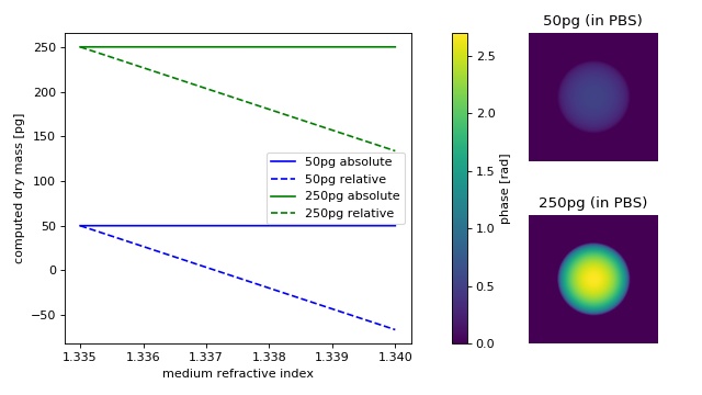
Relative dry mass is the dry mass computed relative to the surrounding medium. If the refractive index of the surrounding medium does not match that of the intracellular fluid (approximately 1.335), then the relative dry mass underestimates the actual dry mass. For a spherical cell, the absolute (corrected) dry mass can be computed as described in the theory section on dry mass computation.
This examples compares the relative dry mass
(drymass.ansphere.relative_dry_mass()) to the
absolute dry mass corrected for a spherical phase object
(drymass.ansphere.absolute_dry_mass_sphere()).
From simulated phase images (projection approach, wavelength 550nm)
of two cell-like spheres with a radius of 10µm and dry masses of
50pg (n≈1.337) and 250pg (n≈1.346), the absolute and relative dry
masses are computed with varying refractive index of the medium.
At the refractive index of phosphate buffered saline (PBS), absolute and relative dry mass are equivalent. As the refractive index of the medium increases, the relative drymass decreases linearly (independent of dry mass), underestimating the actual dry mass.
 1from drymass.anasphere import absolute_dry_mass_sphere, relative_dry_mass
 2import matplotlib
 3import matplotlib.pylab as plt
 4import numpy as np
 5import qpsphere
 6
 7# refraction increment
 8alpha = .18  # [mL/g]
 9
10# general simulation parameters
11model = "projection"
12wavelength = 500e-9  # [m]
13pixel_size = 1.8e-7  # [m]
14grid_size = (200, 200)  # [px]
15
16# sphere parameters
17radius = 10  # [µm]
18center = (100, 100)  # [px]
19
20dry_masses = [50, 250]  # [pg]
21medium_indices = np.linspace(1.335, 1.34, 5)
22
23qpi_pbs = {}
24m_abs = {}
25m_rel = {}
26phase_data = np.zeros(grid_size, dtype=float)
27for m in dry_masses:
28    # initiate results list
29    m_abs[m] = []
30    m_rel[m] = []
31    # compute refractive index from dry mass
32    r_m = radius * 1e-6
33    alpha_m3g = alpha * 1e-6
34    m_g = m * 1e-12
35    n = 1.335 + 3 * alpha_m3g * m_g / (4 * np.pi * (r_m**3))
36    for medium_index in medium_indices:
37        # generate example dataset
38        qpi = qpsphere.simulate(radius=r_m,
39                                sphere_index=n,
40                                medium_index=medium_index,
41                                wavelength=wavelength,
42                                pixel_size=pixel_size,
43                                model=model,
44                                grid_size=grid_size,
45                                center=center)
46        # absolute dry mass
47        ma = absolute_dry_mass_sphere(qpi=qpi,
48                                      radius=r_m,
49                                      center=center,
50                                      alpha=alpha,
51                                      rad_fact=1.2)
52        m_abs[m].append(ma * 1e12)
53        # relative dry mass
54        mr = relative_dry_mass(qpi=qpi,
55                               radius=r_m,
56                               center=center,
57                               alpha=alpha,
58                               rad_fact=1.2)
59        m_rel[m].append(mr * 1e12)
60        if medium_index == 1.335:
61            qpi_pbs[m] = qpi
62
63# plot results
64fig = plt.figure(figsize=(8, 4.5))
65matplotlib.rcParams["image.interpolation"] = "bicubic"
66# phase images
67kw = {"vmax": qpi_pbs[dry_masses[1]].pha.max(),
68      "vmin": qpi_pbs[dry_masses[1]].pha.min()}
69
70ax1 = plt.subplot2grid((2, 3), (0, 2))
71ax1.set_title("{}pg (in PBS)".format(dry_masses[0]))
72ax1.axis("off")
73map1 = ax1.imshow(qpi_pbs[dry_masses[0]].pha, **kw)
74
75ax2 = plt.subplot2grid((2, 3), (1, 2))
76ax2.set_title("{}pg (in PBS)".format(dry_masses[1]))
77ax2.axis("off")
78ax2.imshow(qpi_pbs[dry_masses[1]].pha, **kw)
79
80# overview plot
81ax3 = plt.subplot2grid((2, 3), (0, 0), colspan=2, rowspan=2)
82ax3.set_xlabel("medium refractive index")
83ax3.set_ylabel("computed dry mass [pg]")
84for m, c in zip(dry_masses, ["blue", "green"]):
85    ax3.plot(medium_indices, m_abs[m], ls="solid", color=c,
86             label="{}pg absolute".format(m))
87    ax3.plot(medium_indices, m_rel[m], ls="dashed", color=c,
88             label="{}pg relative".format(m))
89ax3.legend()
90plt.colorbar(map1, ax=ax3, fraction=.048, pad=0.1,
91             label="phase [rad]")
92
93plt.tight_layout()
94plt.subplots_adjust(wspace=.14)
95plt.show()